By: Alessandro Tiberio – Data Engineer
Contributor: Yassir Benhammou PhD. – Data Scientist
Introduction
In Part 1 of this series titled The Business View, we laid out the financial pitfalls that can come from transforming a fragmented data lake into a Retrieval-Augmented Generation (RAG) system, focusing on strategic design and cost-conscious pipeline planning. Now, in Part 2, we shift gears to the technical view. This is really the crux of what data engineers must assemble to build a working RAG factory. If Part 1 answered “why and what,” Part 2 answers “how.” Specifically, we will show how the four pipeline zones introduced in Part 1 (Raw Ingestion, Curated, Embedded, and Indexed) translate into concrete engineering decisions. From data ingestion and orchestration, to document chunking and embedding generation, to loading a vector database and enabling hybrid retrieval, we will walk through what each zone requires to build and keep running reliably.
Recap & Context: In RAG, an LLM is augmented with an external knowledge base so it can retrieve up-to-date, domain-specific information on the fly. The core idea is that we need an indexing pipeline to process and index enterprise data into a vector store and a retrieval pipeline to fetch relevant data for answering queries. In practice, this means data engineers will implement new ETL jobs for unstructured data, integrate vector databases or search services, and orchestrate everything end-to-end. The following sections walk through these components in detail.
Architectural Overview of a RAG Pipeline
At a high level, the solution has two phases: an offline indexing phase where raw data is processed into embeddings and stored in a vector index, and an online query phase where user queries trigger retrieval and generation.
Diagram – Incremental RAG Factory
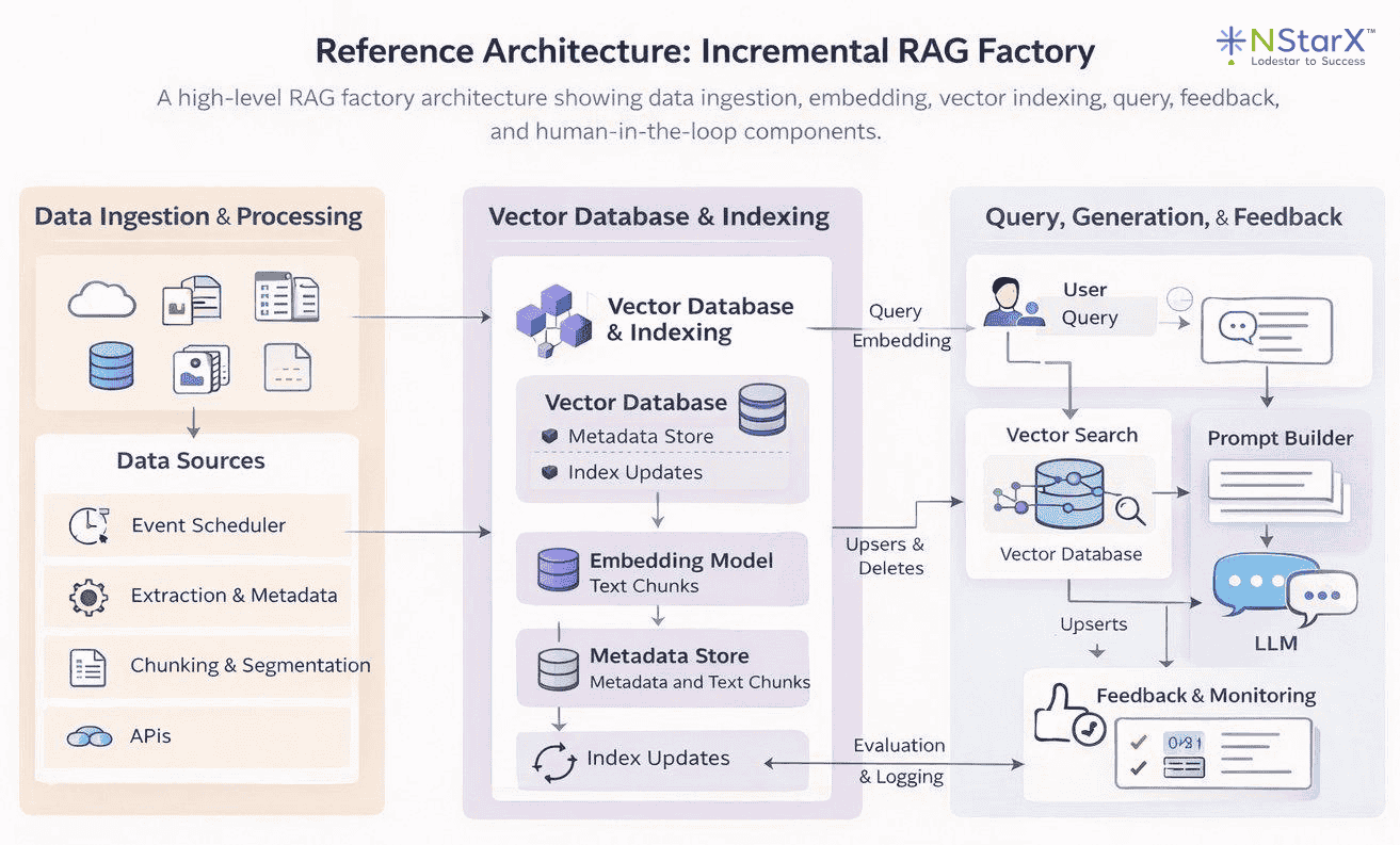
Figure 1: Reference Architecture – Incremental RAG Factory. Source data moves through ingestion, chunking, and embedding before being indexed into a vector database. At query time, user queries are vectorized, relevant chunks are retrieved via similarity search, and results are passed to the LLM for answer generation. A feedback loop keeps the index current over time.
This architecture reflects the four-zone pipeline design introduced in Part 1 of this series: Raw Ingestion, Curated, Embedded, and Indexed Serving. Data ingestion and processing pipelines feed a vector store with embeddings of your organization’s knowledge. When a user query arrives, the system embeds it, performs a similarity search to fetch the most relevant chunks, and passes those as context to the LLM for answer generation. Supporting components include an orchestrator to manage pipeline flows and additional storage for metadata and structured knowledge. With the big picture in mind, let’s break down each component a data engineer must build or integrate.
Data Ingestion and Orchestration
The first step is getting your source data into the pipeline. In a RAG system, source data can range from documents, to database records, to transcripts and so on. It is essentially any knowledge that isn’t already “baked into” the LLM. Data ingestion involves collecting this data, cleaning and normalizing it, and then storing it in a way that downstream processes like embedding generation can consume. Key considerations include connecting to various data sources, handling different file formats, and ensuring data quality.
Connecting Data Sources: Data engineers should set up pipelines to pull in files and records from wherever the knowledge resides. This might mean reading documents from a data lake such as an AWS S3 bucket, querying operational databases for recent records, or using APIs to gather knowledge base articles. In practice, modern toolkits like LangChain or LlamaIndex provide document loaders for many sources, from local files to Confluence pages, which can jumpstart this process. For example, you might use an AWS Glue job or AWS Lambda to regularly scan an S3 location for new documents and load them into memory for processing. The ingestion pipeline should be flexible enough to support multiple formats including PDFs, CSVs, emails, and web pages, with specialized extractors for each data type where needed. Extracting text from complex or scanned documents, for instance, may require an OCR service like Amazon Textract, or an open-source library like Unstructured.io, each of which handles different document types and complexity levels.
Data Cleaning and Enrichment: Once ingested, raw data often needs preprocessing. This includes removing unnecessary content such as boilerplate text or HTML tags, standardizing encodings, and possibly enriching the data with metadata. For example, adding tags like document source, creation date, or access permissions as metadata will be useful later for retrieval filtering. In Part 1, we discussed establishing clean, curated data layers; here, the data engineer ensures each document or record is prepared for chunking. If the data lake already has a “refined zone” or curated layer, the pipeline can draw from there. Otherwise, this step may involve lightweight NLP such as language detection, text normalization, or even translation if needed.
Pipeline Orchestration: Ingestion isn’t a one-off task, it’s an ongoing, automated pipeline. Data engineers must orchestrate these processes to run reliably, whether on a schedule or triggered by events. For example, you might schedule a nightly job to ingest any new or updated documents or use event triggers like an S3 event notification that fires a Lambda when a file is added. Tooling-wise, this could mean using Apache Airflow to manage multi-step workflows or AWS Step Functions to coordinate serverless tasks. The orchestrator handles the sequencing and error handling between components. In a fully AWS-native approach, one could use SageMaker Pipelines or AWS Glue workflows as well. For instance, a SageMaker Pipeline might orchestrate document ingestion with Glue, then invoke a Lambda for chunking, then call an embedding model. The goal is to automate the flow from raw data to indexed vectors in a repeatable way. Robust orchestration also involves monitoring, which could mean using CloudWatch or Airflow’s UI to catch failures and ensure no steps silently break.
Data ingestion and orchestration are the foundation of a reliable RAG pipeline. If the right data doesn’t enter the system cleanly, consistently, and on time, everything downstream — chunking, embeddings, retrieval quality, and answer accuracy — degrades. A data engineer’s job is to turn messy, multi-format knowledge into a governed, repeatable feed that can be indexed safely. Whether you lean on managed services like Kendra connectors or build custom workflows using Lambda, Glue, Step Functions, and/or Airflow, the goal is the same: automate a resilient path from raw sources to fresh, query-ready vectors, with monitoring and failure handling that ensures the pipeline never silently drifts out of date.
Document Chunking Strategies
What Is Chunking and Why Is It Necessary?
RAG systems deal with potentially large documents, but LLMs and vector models have input size limits and work best with focused passages. Data engineers must therefore implement a chunking strategy. Think of it like cutting a long policy manual into individual cards where each card should capture one complete idea, not half a sentence and not an entire chapter. This involves splitting documents into smaller pieces, or chunks, that can be embedded and retrieved individually. Chunking is also not an afterthought, but rather a critical design decision. Too large, and chunks may exceed token limits or dilute relevance; too small, and you lose context or overwhelm the system with too many fragments.
Basic Chunking Approaches: A straightforward strategy is to split text by a fixed size. This could involve splitting text by every N number of characters or tokens; but oftentimes, the latter is the preferred solution since what matters is fitting into model input limits. For example, if you are using an embedding model with a 512-token limit, you might split each document into about 300–500 token chunks to leave some headroom just in case. Another simple approach is splitting by structural markers, which means splitting by paragraph, by sentence, or by headings. Many libraries can split by paragraphs or headings out-of-the-box. Additionally, a common best practice is to allow some overlap between chunks — say 50 tokens or so — so that important context at boundaries isn’t lost. Overlapping chunks means if a sentence straddles two chunks, it will at least fully appear in one of them, reducing the chance of missing relevant info due to unlucky splits.
Intelligent Chunking: Beyond naive splitting, there are also more semantic chunking techniques or “smarter” techniques. The difference here is chunking text into meaningful units rather than by size. “Intelligent” chunking ensures each chunk contains a complete thought or section and is not fragmented, obviously within reason. Advanced pipelines might use NLP (Natural Language Processing) to find sentence boundaries and group sentences until a chunk is at a size threshold. The Unstructured open-source library from Unstructured.io is one widely adopted option which has the ability to implement this “intelligent segmentation,” preserving things like headers, list items, tables, and so on, so that each chunk is self-contained and contextually coherent. The ideal chunk captures a single answerable piece of knowledge such as one FAQ entry, one paragraph about a subtopic, or one section of a policy document. Some systems can also output chunks in structured formats with metadata about data hierarchy (e.g., document → section → subsection). This enables more nuanced retrieval as you could later prioritize chunks from certain sections or versions for certain queries.
Metadata and IDs: No matter the strategy you choose, as chunks are created, it is highly recommended that you tag these chunks with metadata. This typically includes an identifier linking back to the source document, the chunk’s position or section name, and any other useful context such as author, date, topic category, security classification and so on. Metadata is invaluable later for filtered retrieval and for knowing which document a chunk came from. Robust metadata also allows merging or highlighting of the retrieved data in the final answer.
Tooling:Data engineers can use libraries like NLTK or spaCy for sentence tokenization, or the chunking utilities in LangChain which offer options like chunk by tokens with overlap. For more intelligent, structure-aware splitting, the Unstructured open-source library tends to be the go-to option as it handles PDFs, tables, headers, and list items without losing structural context, making it a natural complement to the naive splitters above. On AWS, you could orchestrate chunking with a Lambda function or Glue job after text extraction. The exact implementation can vary, but it’s crucial to document and standardize the chunking approach, because it directly impacts retrieval performance. For instance, smaller chunks mean you will have finer granularity for retrieval, but possibly lower precision as each chunk would have less context. Larger chunks lead to richer context per chunk, but you risk including irrelevant info or missing a specific detail if it’s buried in a big chunk. Part of the blueprint you create for your RAG should include tuning chunk size and overlap based on experimental results for your data.
In Practice:A typical starting point when building a cost-conscious pilot project is to start with naïve chunking of about 200–500 tokens per chunk. This will lead to chunks being roughly a few sentences to a couple of paragraphs, with a 15–30% overlap between chunks. If your documents have clear sections like knowledge base articles with subheadings, you could also choose to chunk by those sections instead. But again, this is really on a case-by-case basis and there is no real “one size fits all” solution. Always make sure to test and verify appropriate chunk size and overlap by testing retrieval during development. Ask sample questions and see if the relevant chunk gets retrieved; if not, adjust your strategy.
Now that your documents have been chunked, we can move to the next major task: converting those text chunks into vector embeddings.
Embedding Generation Pipeline
Once documents are chunked, each chunk of text needs to be transformed into a numerical embedding, which is a vector that captures the semantic content of the text. Think of it like giving each chunk its own postal code. Instead of driving around the neighborhood aimlessly until you find the right house, the system can navigate directly to the correct one based on its postal code (embedding). This is the core of making your data search-friendly and efficient for RAGs. Data engineers must design an efficient pipeline to generate embeddings for all chunks, to futureproof their design. This involves choosing an embedding model, scaling the computation, and managing embedding updates.
What is an Embedding Model:An embedding model is typically a pre-trained LLM that maps text to a high-dimensional vector. Common choices include open-source models like Sentence-BERT or InstructorXL, or API-based models like OpenAI’s text-embedding-ada-002, or cloud offerings like Amazon Titan Embeddings. Key considerations when deciding which model is best for your use case are embedding quality, dimensionality, and the cost versus performance tradeoff. Essentially, does it capture domain-specific semantics, does it support your embedding vector size, and is it in your budget. If you have highly domain-specific text like legal or medical documents, you might consider fine-tuning an embedding model or using one specialized for that domain. That being said, for most use cases, a general model will do just fine with your domain data.
Batch Processing and Scale:Generating embeddings can be a heavy and costly endeavor, especially if you have a large data lake of documents. As such, data engineers should look to leverage distributed computing or batching if they expect a large inflow of data, instead of scaling later as compute costs and processing times start climbing. Tools like Apache Spark or Ray are two frontrunners which let you parallelize embedding computation across a cluster of machines or GPUs. The idea is to distribute chunks across workers, each calling the embedding model concurrently for increased efficiency and speed. If you are self-hosting a model through SageMaker or a TensorFlow/PyTorch service, make sure to load it across multiple machines to avoid a single-machine bottleneck. If you are using a hosted API like Bedrock or OpenAI, you may need to throttle requests or negotiate higher rate limits for large batch jobs. In both cases, the cost-conscious approach is the same. Right-size your compute to the job, process only what has changed, and avoid running full re-embeds when an incremental update will do.
Integration with Orchestration:
The embedding step should be part of the pipeline orchestrator discussed in the ingestion section. For example, in an Airflow DAG you would have a task that takes cleaned and chunked text, sends it to an embedding function, and saves the output vectors. In AWS, you could use SageMaker Batch Transform jobs to handle large embedding tasks in parallel, or AWS Glue with its Spark engine to distribute embedding calls across your data. The right choice depends on the tools already available in your environment, but the principle is the same regardless: never process chunks serially one by one, as that is where big data pipelines grind to a halt. Parallel processing is not just a performance choice here, it’s a cost one too, since idle compute waiting on sequential jobs is money spent for nothing.
Incremental Embedding:
The single most impactful thing you can do to control embedding spend is to never recompute a vector you already have. In practice, this means tracking a content hash or version identifier for each chunk at ingestion time. When a document arrives, compute a hash of its content and compare it against what is already stored. If the hash matches, skip the chunk. Since it has not changed, the existing embedding is still valid. Only chunks that are new, modified, or deleted should flow through the embedding step. If 90% of your document corpus is unchanged in a given run, your embedding cost for that run should reflect roughly 10% of a full recompute, not 100% of it. The mechanics are straightforward: store the content hash alongside each vector in your index. Then, at the start of each pipeline run, check the hash before deciding whether to re-embed. Tools like Apache Airflow make it easy to implement this as a pre-flight check before the embedding task fires. This is not an optimization you bolt on later, it’s something you design in from the start, because retrofitting it onto a pipeline that does not track document versions is painful.
Storing Embeddings Temporarily:
Once computed, embeddings can be written directly into the vector database. However, it is often worth also storing them in intermediate files or a feature store for backup and re-use. For instance, storing embedding vectors in a Parquet file or an embedding store table alongside each chunk ID gives you a portable snapshot of your index. If you later need to switch vector databases or re-compute similarity offline, you are working from what you already have rather than re-generating everything from scratch, which on a large corpus, is a meaningful cost saving. Some organizations take this further by integrating with a feature store to version embeddings as machine learning features. This matters when you update your embedding model, as it lets you compare the old and new embeddings or roll back if the new model underperforms, without losing your previous work.
Verification & Quality:
Every RAG pipeline should include a validation step in the workflow that samples a set of embeddings and checks that they make sense. This can be as simple as taking a known query and running a nearest-neighbor search against a small sample to verify that relevant chunks surface. The goal is to catch issues early, such as a bug producing empty or identical embeddings, before they propagate through to the index. An embedding error that reaches your vector database undetected is not just a quality problem, it is a cost one too. Fixing this problem likely means identifying the affected chunks, re-embedding them, and re-indexing, all of which you have already paid for once and all of which will take additional time and effort.
At this stage, we have embedded our data and produced a large set of vectors, each with their own ID and metadata, collectively representing our knowledge base. The next step is to load these into a vector database, or index, so that the system can find and retrieve the right information when a user asks a question.
Loading and Indexing in a Vector Database
Now that we have our vectors, we need someplace to store them in a way that allows for fast, accurate, and cost-efficient retrieval. This is where a vector database shines. A vector database is a specialized data store optimised for similarity search on high-dimensional vectors. It is the heart of the RAG system’s knowledge base, enabling the retrieval of relevant chunks given a query vector. Data engineers are responsible for deciding which vector store to use, creating an index, loading the embeddings, and planning index refresh strategies to keep everything up to date.
Choosing a Vector Store: When choosing a vector store, as with choosing an embedding model, there are numerous options ranging from fully managed services to self-hosted open source, all coming with their own benefits and shortcomings. Popular choices include Pinecone, Weaviate, Milvus, Vespa, Elastic/OpenSearch, and even extending SQL/NoSQL databases with vector search like Postgres and pgvector, or MongoDB Atlas vector search. On AWS, you have Amazon OpenSearch Service which supports k-NN vector indexes, and Amazon Kendra which offers a high-level retrieval service. Amazon S3 Vectors is also worth considering, integrating a vector index directly into S3 buckets and allowing vector searches without standing up a separate database altogether. The focus here is on patterns rather than endorsing any one product, but the decision should always be grounded in the same questions: can it handle your data at scale, does it support the query capabilities you need, and does it fit your budget.
Index Creation: Once a vector database is chosen, you need to create an index with the right parameters. Key parameters typically include the vector dimension, which must match your embedding size exactly, the distance metric, and any algorithm-specific settings for approximate nearest neighbor search, such as graph complexity for Hierarchical Navigable Small World (HNSW) indexes. OpenSearch’s k-NN plugin, for example, lets you configure these parameters directly, giving you control over the tradeoff between search accuracy, memory footprint, and query latency. In Pinecone or Weaviate, you would specify the metric and shard count at creation time. One important thing to get right from the start: once you define the number of dimensions in your index, every vector you load must match it. It is worth noting that this dimension is determined by the embedding model’s output, not the size of the input chunk. The mismatch risk arises when switching to a different embedding model entirely, which may produce a different output dimension.
Data Loading: Loading millions of embeddings into the index can be time-consuming, so make use of any bulk import features available. Many vector databases support batch upsert operations, and most of the popular ones have this covered. Pinecone and Weaviate have batch APIs, OpenSearch allows bulk HTTP requests, and Postgres with pgvector supports multi-row inserts and direct data copy. Keep a close eye on throughput during this step, as bottlenecks here translate directly into cost on managed services where you are billed for compute time. Parallelizing writes or increasing the number of replicas or shards can help push data in faster. With very large datasets, consider partitioning the index by a meaningful dimension such as data source or ingestion date to keep memory usage manageable, though be aware that this introduces multi-index querying complexity and can add latency at retrieval time.
Metadata and Filtering: As mentioned previously in this paper, whichever vector database you choose, make sure to load metadata alongside your vectors. This allows you to filter search results later by things like document source, date, access permissions, or topic category — which is essential for building a retrieval system that is both accurate and secure. Some enterprise tools like Kendra handle metadata and access control filtering automatically, but if you are using a raw vector database, you need to account for this yourself. OpenSearch, for example, stores the original JSON document alongside the vector, meaning you can include text, title, and tags in that payload and use them for keyword filtering or post-filtering of vector results.
Hybrid Indices: Another pattern worth considering is a hybrid index, which pairs a traditional inverted index for keyword search with a vector index for semantic search. This gives you the best of both worlds, catching exact keyword matches that pure vector search might miss, while still benefiting from semantic similarity for broader queries. OpenSearch supports this natively, combining text relevance and vector similarity in a single query. If you are running separate systems, such as an existing Elasticsearch index for keywords and Pinecone for vectors, you would implement a two-phase retrieval instead, running both searches and merging the results.
Maintaining the Index:The initial load is not the end of the story. New data will arrive, existing data may change, and old data may be deleted entirely. Data engineers must plan for efficient and scalable ways to handle these updates, because a stale index means the LLM will start to return outdated information and the value of the whole system will quietly degrade. In practice, you might maintain a queue of documents that need re-indexing and process it continuously. Managed services like Pinecone, OpenSearch, and Kendra handle a lot of this on the fly, with Kendra able to continuously crawl data sources and update its index with new content. The right approach comes down to two questions: how frequently does your data change, and how fresh does it need to be? If near real-time updates are needed, design your pipeline for streaming inserts. If data changes are infrequent or are not immediately required to be reflected in the query, a perpetual batch re-index is simpler and significantly cheaper.
To recap, up to this point, we have chunked our data, generated embeddings, and loaded those vectors into an indexed database that represents our knowledge base. Now, it is time to put that index to work and actually retrieve relevant information when a user asks a question.
Retrieval and Hybrid Search Mechanisms
Retrieval is where the offline prep work meets the online query. When a user asks a question, the RAG system must fetch the most relevant chunks from the vector index to feed into the LLM. Data engineers need to implement this retrieval process efficiently and consider hybrid strategies that combine semantic search with traditional keyword or database lookups for optimal results.
Vector Similarity Search:Before exploring hybrid strategies, it helps to understand the core retrieval mechanism, which everything else is built on. When a user submits a query, that query is first converted into an embedding, using the same model that was used for your documents. This is intentional as it ensures both the query and the stored chunks live in the same vector space, meaning relevant documents will mathematically be close to the query vector. The pipeline for a query typically follows this path: . The vector database returns the IDs of the top matching chunks along with their similarity scores and any stored metadata. Data engineers often wrap this in an API or service endpoint. For instance, you might build a small microservice that accepts a query, calls the embedding model via Bedrock or a similar API to get the vector, then calls the vector database query interface and returns the top results.
take the query text → embed to vector → query the vector store for top K nearest neighbors
Score Thresholds and Tuning: Part of engineering this retrieval is deciding how many results to retrieve, referred to as K, and whether to apply a minimum similarity score cutoff. A common starting point is K=5 or K=10, which gives the LLM enough context to work with, without overwhelming the prompt. The right number depends heavily on the LLM’s context window. If the model supports 4,000 tokens, you might include 3 to 5 chunks. If it supports 16,000 tokens you can include more, though it is worth remembering that larger context windows cost more per query, so retrieving more than you need is a quiet but consistent cost leak. Some systems dynamically decide how many chunks to include based on similarity scores, pulling in everything above a set threshold rather than a fixed count. Data engineers should expose K and the score threshold as configurable parameters and log retrieval results for continuous tuning. If irrelevant chunks are consistently surfacing as top results, that is a signal to revisit your embedding model, your metadata filters, or both.
Hybrid Retrieval: While vector search is powerful for matching synonyms and related concepts, it can sometimes miss obvious keyword matches or fall short when a query contains rare proper nouns that the embedding space does not capture well. The solution is hybrid retrieval, which combines dense vector-based search with sparse keyword-based methods. The simplest approach is score blending: in a search engine like OpenSearch or Elasticsearch, you can run a single query that includes both a full-text component and a vector component, with the scores combined automatically. Where a single blended query is not possible, two-stage retrieval is the alternative — you run a vector search for semantic hits and a keyword search for literal matches separately, then merge the results by taking a union or selecting whichever result carries the higher confidence score. Some implementations add a re-ranking step on top of this, using a smaller language model or keyword overlap scoring, to further refine relevance before passing results to the LLM. The third and often the most practical approach is metadata filtering: rather than relying solely on the search itself to find the right chunks, you narrow the search space before it runs. If a query is asking about a policy from 2023, filter to only chunks tagged with that year. If a user only has access to certain documents, apply their role-based permissions as a filter before the vector search executes. Amazon Kendra supports this natively through ACL filters, returning only passages the querying user is authorised to see.
Latency Considerations: The retrieval process needs to be fast since it sits directly in the live query path. Vector databases are optimized for millisecond-level similarity searches across millions of vectors, but performance depends heavily on how the index is provisioned. Ensure your index is deployed with enough shards, pods, or memory to avoid I/O bottlenecks, and if you are on a cloud service, choose an instance size that can hold the working index in memory rather than reading from disk on every query. If your pipeline includes additional steps like keyword search or re-ranking, keep them lightweight or run them asynchronously so they do not add to the user-facing response time. Caching is one of the most effective and underused tools for managing latency and cost simultaneously. Caching the results of popular queries, or keeping frequently used query embeddings warm, means the vector search is bypassed entirely for repeat requests, which reduces both response time and the compute cost of running the same search repeatedly.
Fallbacks and Blended Responses: Even a well-tuned RAG system will occasionally find no good vector matches. A user might ask something entirely outside the scope of your indexed documents, or a query might be too ambiguous for the vector search to return anything meaningful. In these cases, the system needs a fallback strategy rather than returning an empty or confusing response. One approach is to switch to direct LLM mode, where the model answers from its own base knowledge when the top similarity score falls below a defined threshold. Another is to always attempt retrieval, but instruct the prompt to respond with something like “I do not have information on that” when the retrieved context is too weak to be useful. Both approaches are valid and the right choice depends on your use case, but the important thing is that the behavior is explicit and intentional. A RAG system that silently returns poor results or hallucinates when retrieval fails is harder to debug and harder to trust than one with a clearly defined fallback.
Testing the Retrieval: Before going to production, test the end-to-end retrieval with a representative set of example queries. For each known query, verify that the retrieved chunks are relevant and that the answers they support are accurate and complete. Involving domain experts in this evaluation is worthwhile, since they are best placed to judge whether the top passages are actually the most useful ones for a given question. Once in production, monitoring is what keeps the system honest over time. Track metrics like the average similarity score of top results and how often queries return nothing above your threshold. These signals tell you when your knowledge base has gaps or when your embedding model is struggling to represent certain types of content accurately.
By implementing robust retrieval and hybrid search where needed, the RAG system can reliably surface the right knowledge at query time. The final step of passing retrieved chunks to the LLM lives in the application layer rather than the data engineering layer, but data engineers should understand how the pieces connect in order to support and debug the full flow when things go wrong.
Putting It All Together and Tooling Considerations
Let’s step back and summarize the RAG factory blueprint from a data engineering perspective. The steps to building your end-to-end RAG pipeline are:
- Ingest and preprocess data from the lake and other sources, ensuring clean, enriched data, ready for AI, and possibly using cloud ETL tools or custom scripts.
- Chunk the data into manageable, semantically meaningful pieces, tagged with metadata for context.
- Generate embeddings for each chunk, using an appropriate model, leveraging distributed compute to handle scale.
- Load those embeddings into a vector index, tuning the index for performance and keeping it refreshed as data changes.
- Handle queries by retrieving relevant chunks via vector similarity or enhanced with hybrid search techniques, to be passed to an LLM for answer generation.
Each of these steps can be implemented with platform-agnostic solutions or with cloud-native services. Data engineers are the glue in this architecture, connecting data storage, ML models, and search infrastructure into one cohesive automated system.
Diagram – AWS-Oriented Example

Figure 2: AWS Alfred reference architecture. A user query is routed through the Alfred Chatbot orchestration layer, which retrieves relevant passages from an Amazon Kendra index fed by an S3 data lake, stores and retrieves conversation history from DynamoDB, and calls Amazon Bedrock for answer generation. Source: AWS Public Sector Blog “Well-rounded technical architecture for a RAG implementation on AWS”.
Tooling Recap:
Let’s briefly recap tools and patterns mentioned to solidify the implementation mindset:
- Ingestion & Orchestration: Apache Airflow/MWAA, AWS Glue, AWS Lambda, AWS Step Functions, Apache NiFi, or even custom Python scripts on a schedule. The key is reliable automation.
- Extraction & Chunking: Unstructured.io library, LangChain loaders & text splitters, AWS Textract for PDFs, Amazon Transcribe for audio to text. Simple regex or text split for basic cases, NLP for advanced.
- Embedding Generation: Hugging Face Transformers for self-managed models, Faiss library if doing local embedding and ANN search, Bedrock’s Titan Embeddings API, OpenAI embeddings API, Cohere embeddings, and so on. Use distributed computing like Spark, Ray, Dask or even something like SageMaker for scaling up.
- Retrieval & App Integration: Aside from the vector DB query itself, libraries like LangChain or LlamaIndex can simplify the retrieval and LLM integration in code. They allow you to define a retriever that encapsulates the vector search and then automatically format the LLM prompt with retrieved texts. Data engineers may collaborate with ML engineers to embed such libraries into applications. On AWS, Bedrock plus Kendra can be combined with relatively few lines of glue code as these are both natively managed solutions.
- Vector Store: Depending on your requirements, OpenSearch Service, Amazon Kendra, Pinecone, Weaviate, Milvus, Qdrant, pgvector on Postgres, or even the emerging S3 Vector indexing. Each has pros and cons on cost, complexity, and capabilities. For example a managed service like Kendra offers built-in connectors and auth, but an open-source solution might offer more customizability.
Conclusion
Building a RAG factory from your data lake is a complex but well-structured engineering challenge. It requires knowledge of data pipelines, NLP, search technology, and ML orchestration. In this guide, we walked through how a data engineer can approach it step by step, ingesting and preparing data, chunking it for retrieval, generating embeddings to create a semantic index, and enabling robust retrieval mechanisms to feed an LLM with the right knowledge on demand.
By following this blueprint, organisations can move from simply having a data lake to actively putting that data to work in intelligent, context-aware AI applications. The data engineer’s role in this is central. They build and maintain the factory that continually transforms raw data into vectorized knowledge, keeping the AI grounded in what is actually true rather than what the base model has guessed. With the right design choices and tooling, whether that is AWS managed services or open-source alternatives, this pipeline can run efficiently and scale without spiralling costs.
Start small. Pick a subset of your data, something that is relevant and readily required. Build the pipeline end-to-end, and validate that retrieval works before expanding scope. This way, any pilot project you engage in won’t go stale after a week. This is a fast-moving space, and the tools will keep improving, but the principles covered here are stable. A well-built foundation is what separates a RAG system that delivers lasting value, from one that becomes another abandoned pilot project.
References
- Amazon Web Services. “What is RAG? Retrieval-Augmented Generation AI Explained.” https://aws.amazon.com/what-is/retrieval-augmented-generation/
- Amazon Web Services. “Build a RAG data ingestion pipeline for large-scale ML workloads.” https://aws.amazon.com/blogs/big-data/build-a-rag-data-ingestion-pipeline-for-large-scale-ml-workloads/
- Amazon Web Services. “Well-rounded technical architecture for a RAG implementation on AWS.” https://aws.amazon.com/blogs/publicsector/well-rounded-technical-architecture-for-a-rag-implementation-on-aws/
- Amazon Web Services. “Hybrid Search with Amazon OpenSearch Service.” https://aws.amazon.com/blogs/big-data/hybrid-search-with-amazon-opensearch-service/
- Amazon Web Services. “Introducing Amazon S3 Vectors: First cloud storage with native vector support at scale.” https://aws.amazon.com/blogs/aws/introducing-amazon-s3-vectors-first-cloud-storage-with-native-vector-support-at-scale/
- Amazon Web Services. “Amazon S3 Vectors now generally available with increased scale and performance.” https://aws.amazon.com/blogs/aws/amazon-s3-vectors-now-generally-available-with-increased-scale-and-performance/
- lakeFS. “RAG Pipeline: Example, Tools & How to Build It.” https://lakefs.io/blog/what-is-rag-pipeline/
- Ajay Jetty. “A RAG Pipeline (with DataLake) to automate customer support for a consumer SaaS App.” https://ajayjetty.medium.com/a-rag-pipeline-with-datalake-to-automate-customer-support-for-a-consumer-saas-app-e878a05ca78d
- Ray Munene. “Building Retrieval-Augmented Generation (RAG) Pipelines on AWS: A Production-Ready Guide.” https://medium.com/@raymunene/building-retrieval-augmented-generation-rag-pipelines-on-aws-a-production-ready-guide-2b16cd2ccec3
- Multimodal. “RAG Pipeline Diagram: How to Augment LLMs With Your Data.” https://www.multimodal.dev/post/rag-pipeline-diagram
- Unstructured. “Chunking Strategies for RAG: Best Practices and Key Methods.” https://unstructured.io/blog/chunking-for-rag-best-practices
- Unstructured. “Unstructured’s Preprocessing Pipelines Enable Enhanced RAG Performance.” https://unstructured.io/blog/unstructured-s-preprocessing-pipelines-enable-enhanced-rag-performance
- pgvector. “Open-source vector similarity search for Postgres.” https://github.com/pgvector/pgvector
- OpenSearch. “Hybrid Search.” https://docs.opensearch.org/latest/vector-search/ai-search/hybrid-search/index/
- OpenSearch. “Vector Search.” https://docs.opensearch.org/latest/vector-search/